Example Applications
Background
spacejam can be used to simulate a wide range of physical systems. To
accomplish this, we provide an integration suite of implicit solvers that draw
from the first three orders of the Adams-Moulton methods. These methods can
be accessed from spacejam.integrators and each use the root finding
Newton-Raphson method with an initial forward Euler guess. We will now describe
each implicit scheme and how to go about using it with spacejam.
(s = 0) Method
As we saw in Numerical Integration: A brief crash couse, this is a numerical scheme to solve the implicit equation:
by re-casting it as the root finding problem:
In 1D, the Newton-Raphson method successively finds better and better approximations to the root of a function \(f(x)\) in the following way:

- Make a guess next to one of the roots you want
- Draw the corresponding tangent line (red) at this guess evaluated on the original function (blue)
- Trace this tangent line to where it intercepts the x-axis
- Make this intercept your new guess
- Rinse and repeat until your latest guess is close enough (your tolerance) to the root you wanted to approximate in the first place
The equation for this can be quickly derived by solving for the next root iterate \(x_{n+1}\) from the definition of the derivative:
This is naturally extended to vector functions that accept multi-valued input by using the multi-variable version of the derivative, the Jacobian \(\b J\):
where:
For these examples, \(m=k\), \(\b f = \b {\dot X}_n = [\dot x_1, \dot x_2, \cdots, \dot x_m]_n\), \(1 \le i,j \le k\) .
Applying this to our backward Euler equation:
Here, \((i)\) and \((i+1)\) have been used to avoid confusion with the \(n\) and \(n+1\) iterate used in the 1D example above, and the root to this equation is the solution \(\b X_{n+1}\) to our original implicit equation. The Jacobian \(\b J\) is hiding inside of \(\b D\) and we can make it show itself by just performing the multi-variable derivative that is required of the Newton-Raphson method:
where \(\b I\) is the identity matrix. All that is needed now is an initial guess for \(\b X_{n+1}^{(0)}\) to jump start Newton’s method. A single forward Euler step should do:
In this framework, both the real and dual part of the dual object returned by
spacejam will be used. To summarize:
- The user supplies the system of equations \(\b {\dot X}_{n}\) and initial conditions \(\b {\dot X}_{n}^{(0)}\) .
- The user implements the integration scheme using the real part returned
from
spacejamfor \(\b {\dot X}_{n}^{(i)}\) and the dual part as \(\b{J}\left[\left(\b {\dot X}_{n+1}\right)^{(i)}\right]\) .
(s = 1) Method
A similar implementation can be made with the next order up in this family of implicit methods. In this scheme we have:
Applying the same treatment of turning this into a root finding problem and applying Newton’s method gives the similar result:
In this new scheme, \(\b D\) has an extra factor of \(1/2\) on its
Jacobian in the backward and now spacejam will also be computing
\(\b {\dot X_n}\).
(s = 2) Method
In this final scheme we have:
The corresponding \(\b g\) and \(\b D\) are then:
Note
Each of the three methods above are implemented in
spacejam.integrators. The tolerance determining when to end
Newton-Raphson iterations and the break point in number of iterations
can also respectively be controlled by the keyword arguments X_tol
and i_tol in all integrator functions.
We demonstrate each method in our example systems below.
Astronomy Example
Background
In this example, we will integrate the orbits of a hypothetical three-body star-planet-moon system. This exercise is motivated by the first potential discovery of an exomoon made not too long ago.
In 2D Cartesian coordinates, the equations of motion that govern the orbit of body \(A\) due to bodies \(B\) and \(C\) are:
where the following definitions are given:
- \((x_i, y_i)\): positional coordinates of body \(i\), with mass \(m_i\)
- \((v_{x_i}, v_{y_i})\): components of body \(i\)‘s velocity
- \(d_{ij}\): distance between body \(i\) and body \(j\)
- \(G\): Universal Gravitational Constant (as far as we know)
We will be using an external package (astropy) that is not included in
spacejam for this demonstration. This step is totally optional, but it
makes using units and physical constants a lot more convenient.
Initial Conditions
For this toy model, let’s place a \(10\) Jupiter mass exoplanet \(0.01\ \text{AU}\) to the left of a sun-like star, which we place at the origin. Let’s also have this exoplanet orbit this star with the typical Keplerian velocity \(v = \sqrt{GM/r}\), starting in the negative \(y\) direction, where \(M\) is the mass of the star and r is the distance of this exoplanet from its star.
Next, let’s place an exomoon with \(1/1000\) th the mass of the exoplanet about \(110,000\ \text{km}\) to the left of this exoplanet. This ensures that the exomoon is within its gravitational sphere of influence. Let’s also have this exomoon start moving with Keplerian speed in the negative \(y\) direction. note: this would be the sum of the exoplanet’s velocity and the Keplerian speed of the moon due to just the gravitational influence of the exoplanet.
Finally, let’s pick a time step that goes something like a tenth of the time it would initially take the exomoon to fall straight into the planet if it didn’t happen to have any Keplerian speed. To a certain extent, this choice is pretty arbitrary because of implicit schemes’ relative insensitivity to time step size relative to those for explicit schemes, but our implicit solving implementation does partially rely on an explicit scheme, so it’s still important to consider.
import numpy as np
from astropy import units as u
from astropy import constants as c

# constants
solMass   = (1 * u.solMass).cgs.value
solRad    = (1 * u.solRad).cgs.value
jupMass   = (1 * u.jupiterMass).cgs.value
jupRad    = (1 * u.jupiterRad).cgs.value
earthMass = (1 * u.earthMass).cgs.value
earthRad  = (1 * u.earthRad).cgs.value
G         = (1 * c.G).cgs.value
AU        = (1 * u.au).cgs.value
year      = (1 * u.year).cgs.value
day       = (1 * u.day).cgs.value
earth_v   = (30 * u.km/u.s).value
moon_v    = (1 * u.km/u.s).cgs.value

# mass ratio of companion to secondary
q              = 0.001
# primary
host_mass      = solMass
host_rad       = solRad
# secondary
scndry_mass    = 10*jupMass
scndry_rad     = 1.7*jupRad
scndry_x       = -0.01*AU
scndry_y       = 0.0
scndry_vx      = 0.0
scndry_vy      = -np.sqrt(G*host_mass/np.abs(scndry_x)) # assuming Keplerian for now
# companion
cmpn_mass      = q*scndry_mass
cmpn_rad       = 0.3*scndry_rad
hill_sphere    = np.abs(scndry_x) * (scndry_mass / (3*host_mass))**(1/3)
cmpn_x         = scndry_x - 0.5 * hill_sphere
cmpn_y         = scndry_y
cmpn_vx        = 0.0
cmpn_vy        = scndry_vy - np.sqrt(G*scndry_mass/(0.5 * hill_sphere))

m_1 = host_mass # host star
m_2 = scndry_mass #m_1 / 5000 # hot jupiter
m_3 = cmpn_mass  # companion

# m1: primary (hardcoded)
x_1  =  0.0
y_1  =  0.0
vx_1 =  0.0
vy_1 =  0.0

# m2: secondary
x_2  = scndry_x
y_2  = scndry_y # doesn't matter where it starts on y because of symmetry of system
vx_2 = scndry_vx
vy_2 = scndry_vy # assuming Keplerian for now

# m3: companion
x_3  = cmpn_x
y_3  = cmpn_y
vx_3 = cmpn_vx
vy_3 = cmpn_vy

# characteristic timescale set by secondary's orbital timescale
T0 = 2*np.pi*np.sqrt(np.abs(scndry_x)**3/(G*m_1))
tmax  = 2.5*T0

uold_1 = np.array([x_1, y_1, vx_1, vy_1])
uold_2 = np.array([x_2, y_2, vx_2, vy_2])
uold_3 = np.array([x_3, y_3, vx_3, vy_3])

m1_coord = uold_1
m2_coord = uold_2
m3_coord = uold_3

r0 = np.sqrt( (uold_3[0] - uold_2[0])**2 + (uold_3[1] - uold_2[1])**2 )
v0 = np.sqrt(uold_3[2]**2 + uold_3[3]**2)
f = -1
h = 10**(f) * r0 / v0
N = 1500 # number of steps to run sim

# Store initial positions and velocities
uold_1 = np.array([x_1, y_1, vx_1, vy_1]) # star
uold_2 = np.array([x_2, y_2, vx_2, vy_2]) # exoplanet
uold_3 = np.array([x_3, y_3, vx_3, vy_3]) # exomoon
Equations of Motion
The system of differential equations governing our system look like:
def f(x, y, vx, vy, uold_b=None, mb=0, uold_c=None, mc=0):
    # position and velocity
    r_a = np.array([x, y])
    v_a = np.array([vx, vy])

    r_b = uold_b[:2]
    r_c = uold_c[:2]

    # position vector pointing from one of the two masses to m_i
    d_ab = np.linalg.norm(r_b - r_a)
    d_ac = np.linalg.norm(r_c - r_a)

    # calulating accelerations
    gx = G*mb/d_ab**3 * (r_b[0] - x) + (G*mc/d_ac**3) * (r_c[0] - x)
    gy = G*mb/d_ab**3 * (r_b[1] - y) + (G*mc/d_ac**3) * (r_c[1] - y)

    # return derivatives
    f1 = vx
    f2 = vy
    f3 = gx
    f4 = gy
    return np.array([f1, f2, f3, f4])
Simulation
Our toy model can now be run with spacejam and its included suite of
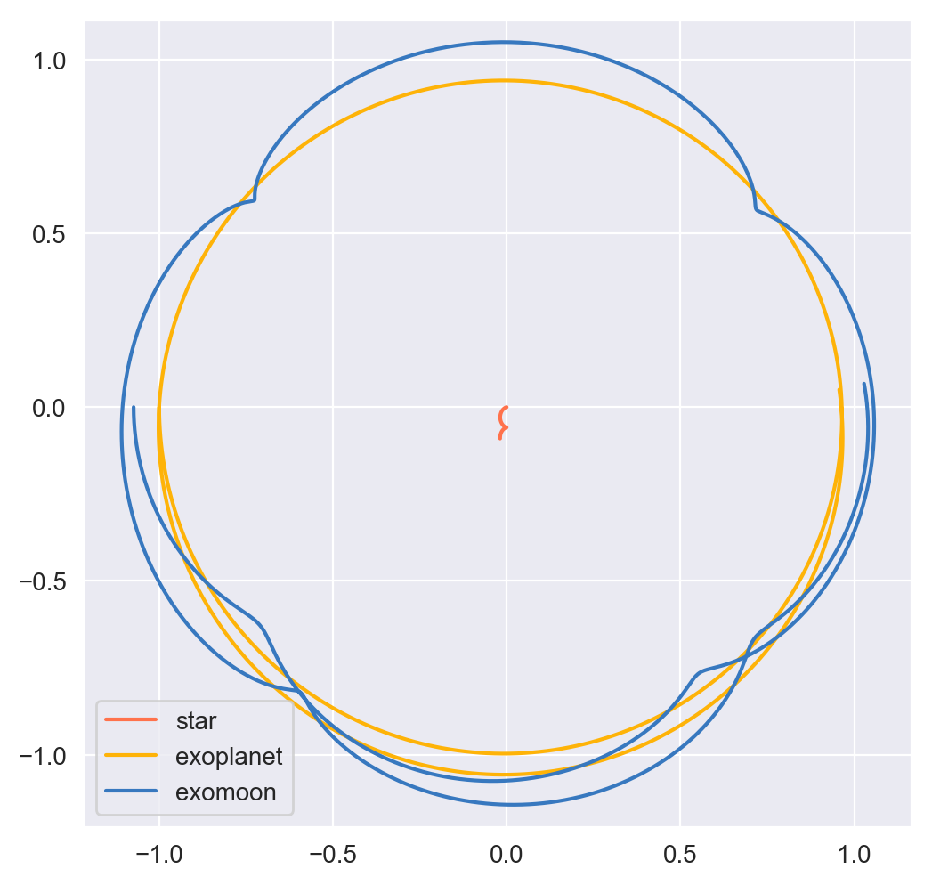
integrators to produce the following orbits.
(s = 0)
import spacejam as sj

X_1 = np.zeros((N, uold_1.size))
X_1[0] = uold_1
X_2 = np.zeros((N, uold_2.size))
X_2[0] = uold_2
X_3 = np.zeros((N, uold_3.size))
X_3[0] = uold_3

for n in range(N-1):
    kwargs_1 = {'uold_b': X_2[n], 'mb': m_2, 'uold_c': X_3[n], 'mc': m_3}
    X_1[n+1] = sj.integrators.amso(f, X_1[n], h=h, kwargs=kwargs_1)

    kwargs_2 = {'uold_b': X_1[n], 'mb': m_1, 'uold_c': X_3[n], 'mc': m_3}
    X_2[n+1] = sj.integrators.amso(f, X_2[n], h=h, kwargs=kwargs_2)

    kwargs_3 = {'uold_b': X_1[n], 'mb': m_1, 'uold_c': X_2[n], 'mc': m_2}
    X_3[n+1] = sj.integrators.amso(f, X_3[n], h=h, kwargs=kwargs_3)

    # stop iterating if Newton-Raphson method does not converge
    if X_1[n+1] is None or X_2[n+1] is None or X_3[n+1] is None:
        break

Note
Axes are scaled by the initial distance of the exoplanet from its host star and oriented in the usual XY fashion.
This integration scheme actually fails partway through the simulation.
spacejam provides the following suggestions to fix this in its error
message:
SystemExit:
Sorry, spacejam did not converge for s=0 A-M method.
Try adjusting X_tol, i_tol, or using another integrator.
We will follow the last suggestion and use the higher order s=1 scheme instead.
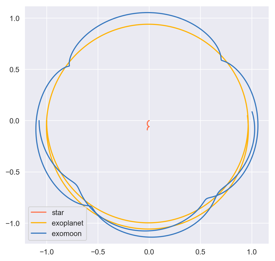
(s = 1)
X_1 = np.zeros((N, uold_1.size))
X_1[0] = uold_1
X_2 = np.zeros((N, uold_2.size))
X_2[0] = uold_2
X_3 = np.zeros((N, uold_3.size))
X_3[0] = uold_3

for n in range(N-1):
    kwargs_1 = {'uold_b': X_2[n], 'mb': m_2, 'uold_c': X_3[n], 'mc': m_3}
    X_1[n+1] = sj.integrators.amsi(f, X_1[n], h=h, kwargs=kwargs_1)

    kwargs_2 = {'uold_b': X_1[n], 'mb': m_1, 'uold_c': X_3[n], 'mc': m_3}
    X_2[n+1] = sj.integrators.amsi(f, X_2[n], h=h, kwargs=kwargs_2)

    kwargs_3 = {'uold_b': X_1[n], 'mb': m_1, 'uold_c': X_2[n], 'mc': m_2}
    X_3[n+1] = sj.integrators.amsi(f, X_3[n], h=h, kwargs=kwargs_3)

    # stop iterating if Newton-Raphson method does not converge
    if X_1[n+1] is None or X_2[n+1] is None or X_3[n+1] is None:
        break
It works! Let’s go up another order.
(s = 2)
X_1 = np.zeros((N, uold_1.size))
X_1[0] = uold_1
X_2 = np.zeros((N, uold_2.size))
X_2[0] = uold_2
X_3 = np.zeros((N, uold_3.size))
X_3[0] = uold_3

# This method requires the 2nd step as well to get started. Will
# just use a forward Euler guess for this
kwargs_1 = {'uold_b': X_2[0], 'mb': m_2, 'uold_c': X_3[0], 'mc': m_3}
ad = sj.AutoDiff(f, X_1[0], kwargs=kwargs_1)
X_1[1] = X_1[0] + h*ad.r.flatten()

kwargs_2 = {'uold_b': X_1[0], 'mb': m_1, 'uold_c': X_3[0], 'mc': m_3}
ad = sj.AutoDiff(f, X_2[0], kwargs=kwargs_2)
X_2[1] = X_2[0] + h*ad.r.flatten()

kwargs_3 = {'uold_b': X_1[0], 'mb': m_1, 'uold_c': X_2[0], 'mc': m_2}
ad = sj.AutoDiff(f, X_3[0], kwargs=kwargs_3)
X_3[1] = X_3[0] + h*ad.r.flatten()

for n in range(1, N-1):
    kwargs_1 = {'uold_b': X_2[n], 'mb': m_2, 'uold_c': X_3[n], 'mc': m_3}
    X_1[n+1] = sj.integrators.amsii(f, X_1[n], X_1[n-1],
                                    h=h, kwargs=kwargs_1)

    kwargs_2 = {'uold_b': X_1[n], 'mb': m_1, 'uold_c': X_3[n], 'mc': m_3}
    X_2[n+1] = sj.integrators.amsii(f, X_2[n], X_2[n-1],
                                    h=h, kwargs=kwargs_2)

    kwargs_3 = {'uold_b': X_1[n], 'mb': m_1, 'uold_c': X_2[n], 'mc': m_2}
    X_3[n+1] = sj.integrators.amsii(f, X_3[n], X_3[n-1],
                                    h=h, kwargs=kwargs_3)

    # stop iterating if Newton-Raphson method does not converge
    if X_1[n+1] is None or X_2[n+1] is None or X_3[n+1] is None:
        break
Note
All plots for this example were styled with the external package seaborn and created with the following snippet below:
import matplotlib.pyplot as plt
import seaborn as sns

sns.set_style('darkgrid')

fig, ax = plt.subplots(figsize=(6, 6))
ax.set_aspect('equal', 'datalim')

# normalize plot axes
a_0 = np.linalg.norm(m2_coord)

# custom colors
c1 = sns.xkcd_palette(["pinkish orange"])[0]
c2 = sns.xkcd_palette(["amber"])[0]
c3 = sns.xkcd_palette(["windows blue"])[0]

ax.plot(X_1[:,0]/a_0, X_1[:,1]/a_0, c=c1, label='star')
ax.plot(X_2[:,0]/a_0, X_2[:,1]/a_0, c=c2, label='exoplanet')
ax.plot(X_3[:,0]/a_0, X_3[:,1]/a_0, c=c3, label='exomoon')

ax.legend()
Static images can be a bit difficult to interpret, so we also included a stylized movie for the final plot.
Note
Everything is still scaled by the initial distance of the exoplanet from its star.
An analysis of the change in total energy and angular momentum of the system each step in the simulation would be a good diagnostic to see which integration scheme is actually giving the most accurate results.
Now we turn to a completely different example that can also be handled with
spacejam.
Ecology Example
Background
In this example, we look at a popular system of differential equations used to describe the dynamics of biological systems where two sets of species (predator and prey) interact. The population of each can be tracked with:
where,
- \(x\): number of prey
- \(y\): number of predators
- \(\dot x\) and \(\dot y\): instantaneous growth rate of the prey and predator populations, respectively
- \(\alpha, \beta, \delta, \gamma\): parameters describing interactions of the two species
Initial Conditions
We will test this system with the initial conditions that are known to produce a stable system.
import numpy as np

N = 1000
h = .01 # timestep
X_0 = np.array([2., 1.]) # initial population conditions ([prey, predator])
X = np.zeros((N, X_0.size))
X[0] = X_0
Equations of population growth
The system can be created with the following:
def f(x1, x2, alpha=4., beta=4., delta=1., gamma=1.):
    f1 = alpha*x1 - beta*x1*x2
    f2 = delta*x1*x2 - gamma*x2
    return np.array([f1, f2])
Simulation
Running this with the suite of integrators in spacejam then gives the
following:
(s = 0) Method
for n in range(N-1):
    X[n+1] = sj.integrators.amso(f, X[n], h=h, X_tol=1E-14)
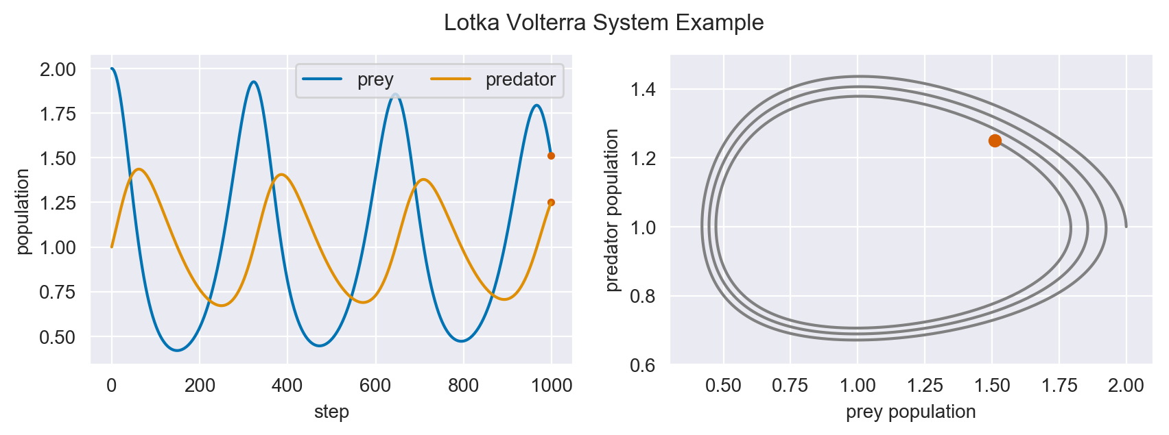
In the plots above, we see the hallmark numerical damping of implicit schemes, which causes the overall prey and predator population to artificially decrease each step. This is especially apparent in the phase plot of the two populations where an in-spiral is present. Let’s see if this is still the case for high order schemes.
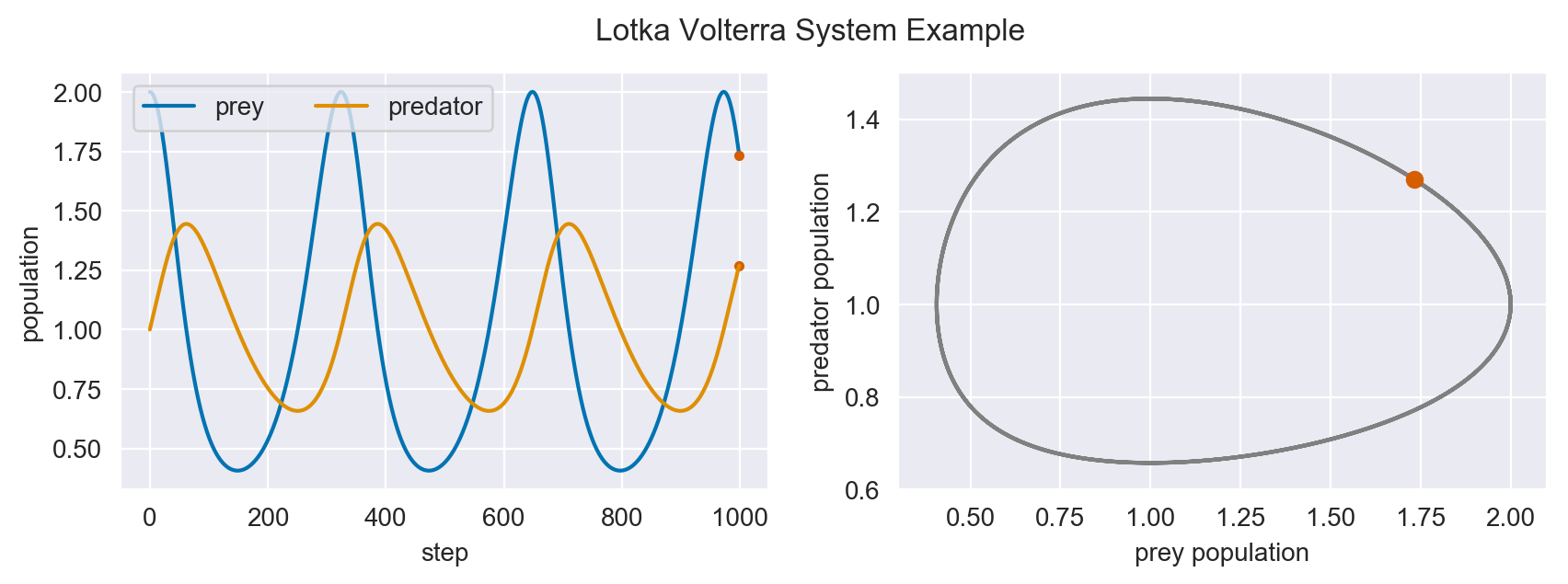
(s = 1) Method
for n in range(N-1):
    X[n+1] = sj.integrators.amsi(f, X[n], h=h, X_tol=1E-14)
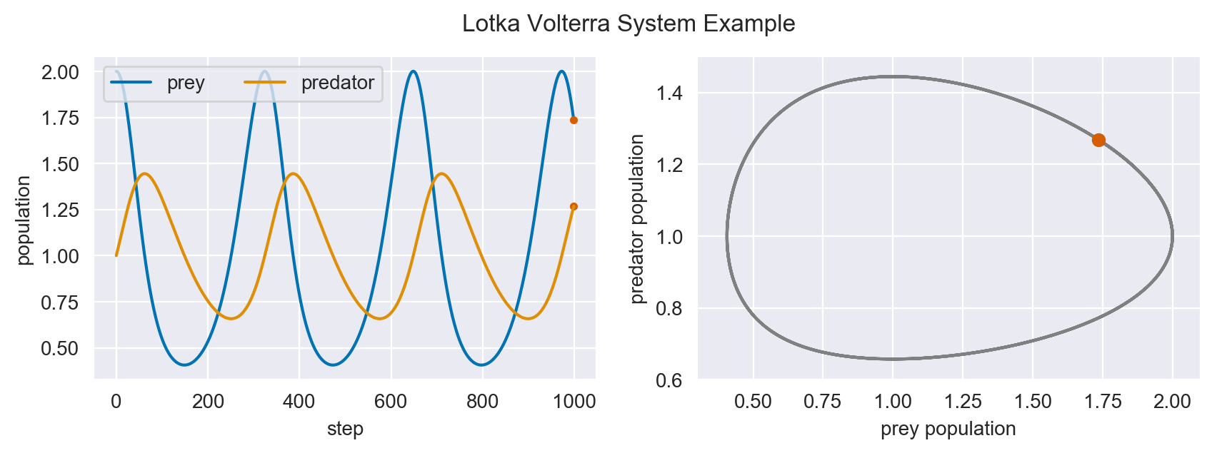
The spiral is gone and the ecological system is stable!
(s = 2) Method
for n in range(N-1):
    X[n+1] = sj.integrators.amsi(f, X[n], h=h, X_tol=1E-14)
As expected, the higher order scheme maintains stability as well, assuming same initial conditions. Below is an animation of the s=0 implicit simulation of this system tracking the in-spiraling of the phase plot.
Note
All plots for this example were made with the following snippet below:
# plot setup
sns.set_palette('colorblind')
sns.set_color_codes('colorblind')
fig, axes = plt.subplots(1, 2, figsize=(10, 3))
ax1, ax2 = axes

# solution plot
n = np.arange(N)
prey = X[:, 0]
pred = X[:, 1]

ax1.plot(n, prey, label='prey')
ax1.plot(n[-1], prey[-1], 'r.')
ax1.plot(n[-1], pred[-1], 'r.')
ax1.plot(n, pred, label='predator')
ax1.set_xlabel('step')
ax1.set_ylabel('population')
ax1.legend(ncol=2)

# phase plot
ax2.plot(prey, pred)
ax2.plot(prey[-1], pred[-1], 'r.')
ax2.set_xlabel('prey population')
ax2.set_ylabel('predator population')
ax2.set_xlim(0.3, 2.1)
ax2.set_ylim(0.6, 1.5)

plt.suptitle('Lotka Volterra System Example')
Movies were made with matplotlib.animation using its ffmeg
integration. We have included a sample notebook demoing this and the
above examples in our main repo.